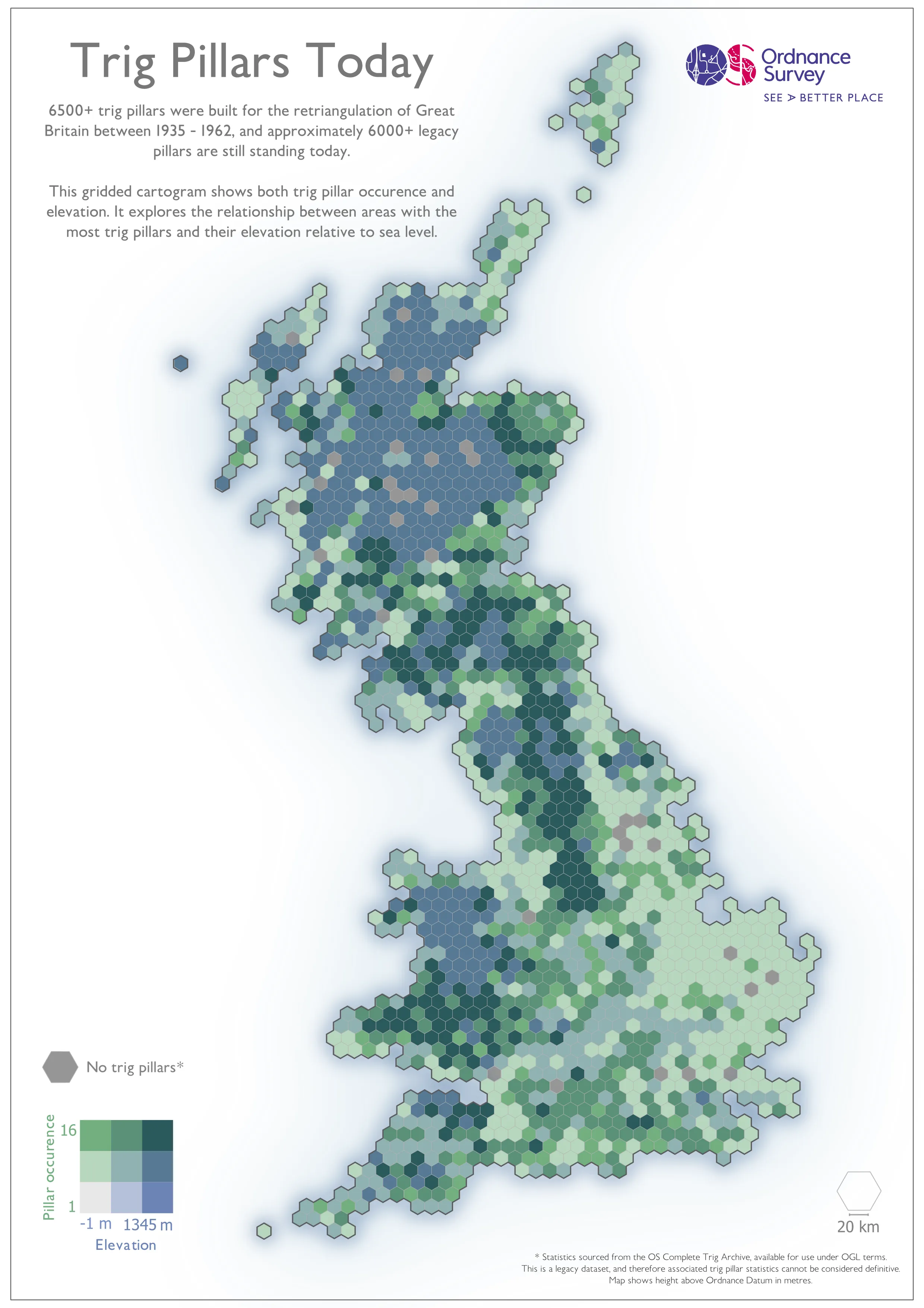
Hexagonal cartogram, illustrating both trig pillar occurrence and elevation across Great Britain
Hexagonal cartogram, illustrating both trig pillar occurrence and elevation across Great Britain
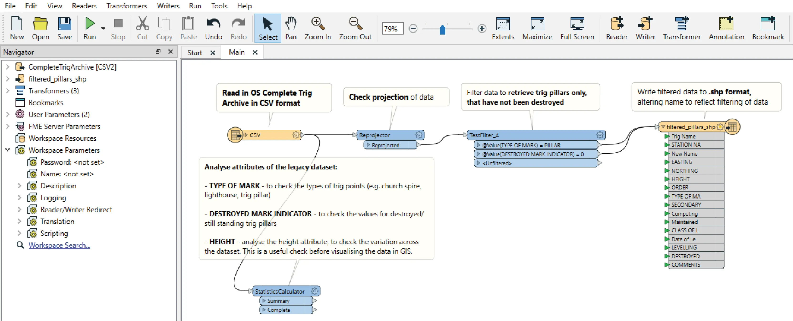
FME Workbench, used to filter the OS Complete Trig Archive
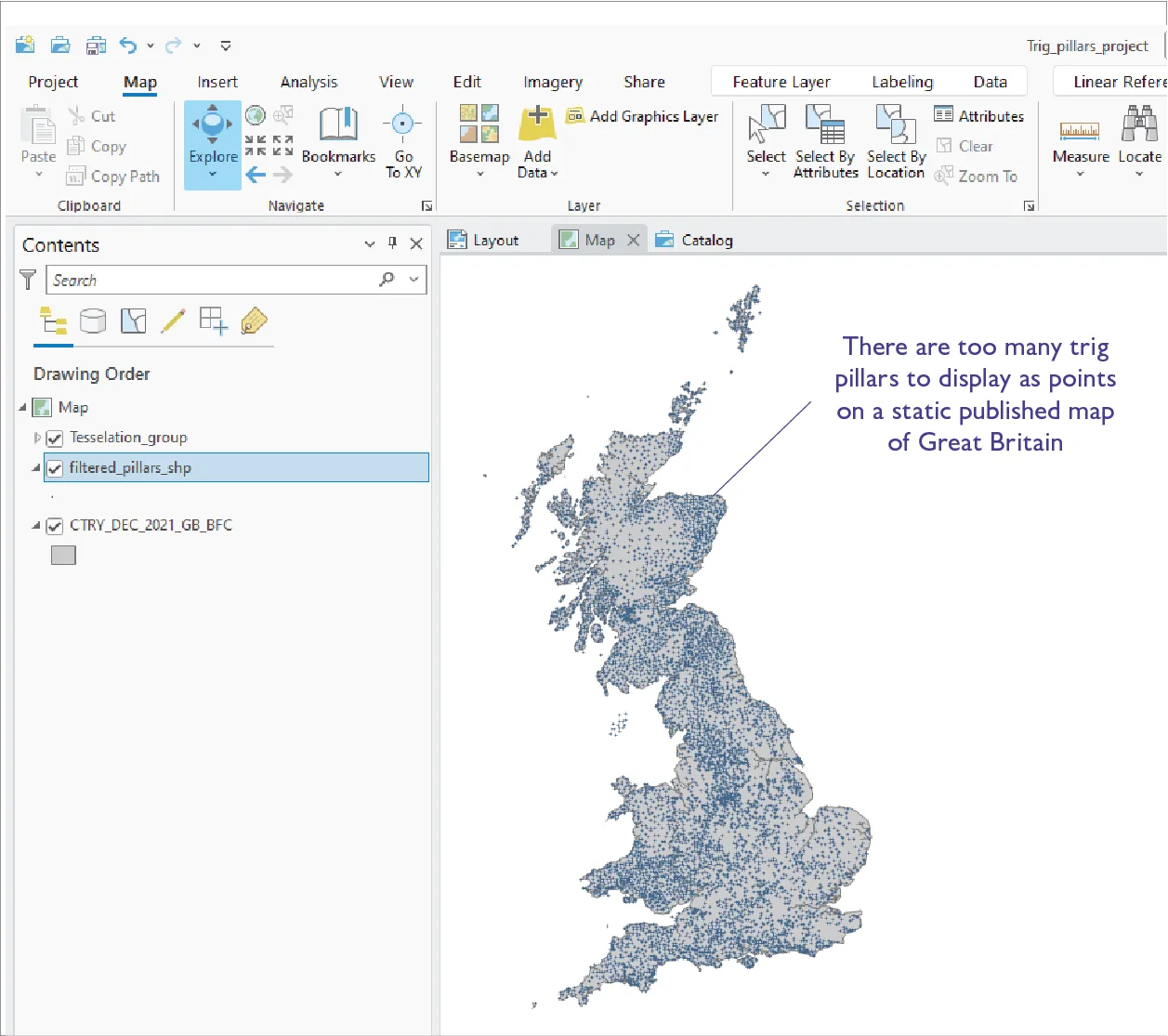
Placing the data in ArcGIS Pro illustrates the density of the data to work with
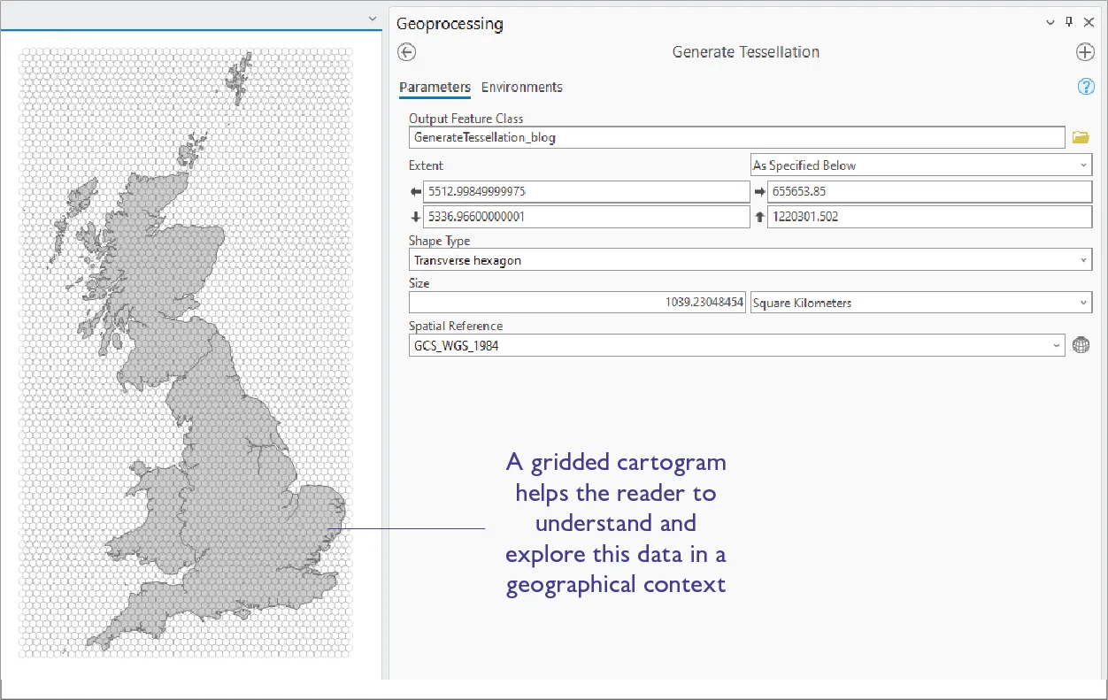
Using the Generate Tessellation tool in ArcGIS Pro to create a hexagonal grid across Great Britain
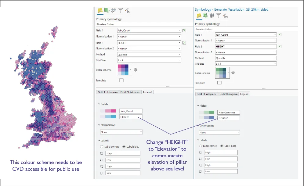
By altering the legend, we can communicate that height actually means elevation above sea level in this context
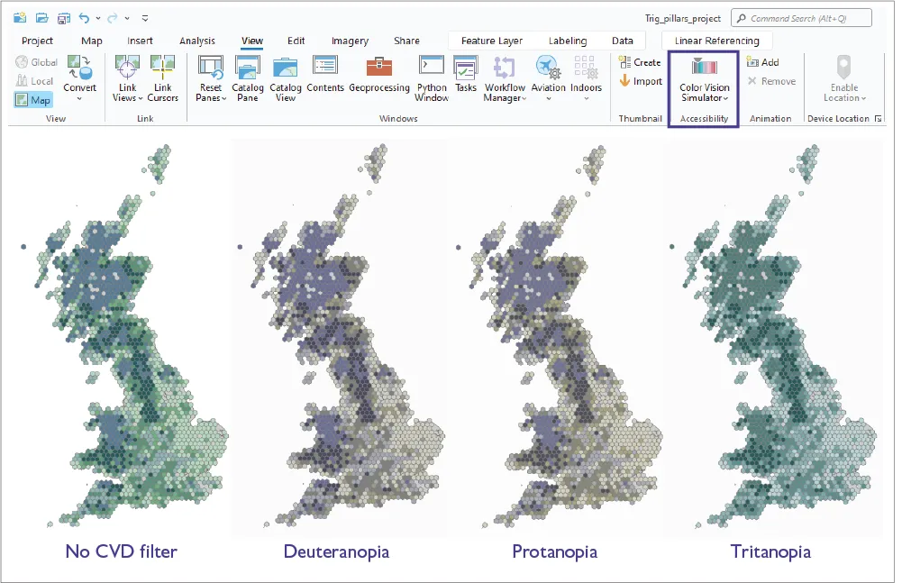
ArcGIS Pro has some helpful CVD filters, that should be used to check your colour scheme before sharing your design
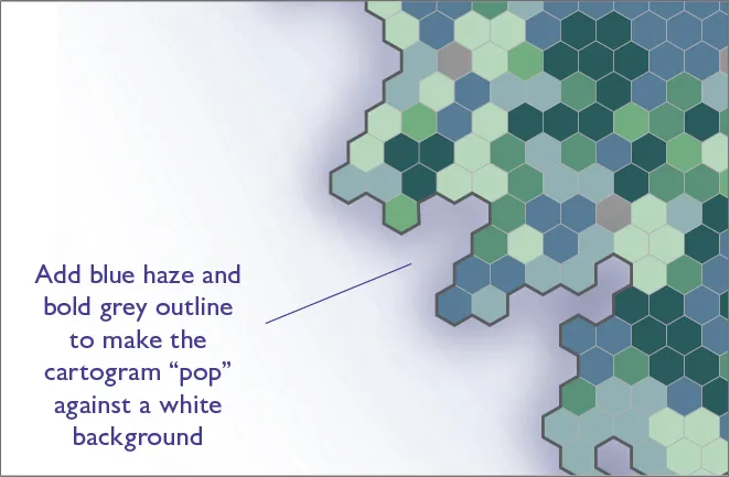
Adding an outline to the map