> For the complete documentation index, see [llms.txt](https://docs.os.uk/more-than-maps/llms.txt). Markdown versions of documentation pages are available by appending `.md` to page URLs; this page is available as [Markdown](https://docs.os.uk/more-than-maps/geographic-data-visualisation/geodataviz-assets/how-did-i-make-that/apollo-11-landing.md).
# Apollo 11 Landing
On 20 July 1969 at 20:17 GMT, Apollo 11 touched down on the moon. Six hours later Neil Armstrong became the first person to step onto the lunar surface. It was a monumental achievement for humanity.
The Moon landing was part of the Apollo programme, which started in 1966 and led to 11 astronauts, including Buzz Aldrin, to walk on the moon after Neil. A huge part of the mission was working out where to safely touch down. NASA’s Apollo Site Selection Board identified five potential landing sites for Apollo 11 based on the following criteria:
* The site needed to be smooth, with relatively few craters.
* Have approach paths free of large hills, tall cliffs or deep craters that might confuse the landing radar and cause it to issue incorrect readings.
* Be reachable with a minimum amount of propellant.
* Provide the Apollo spacecraft with a free-return trajectory, one that would allow it to coast around the Moon and safely return to Earth without requiring any engine firings should a problem arise on the way to the Moon.
* Have good visibility during the landing approach, meaning that the Sun would be between 7 and 20 degrees behind the landing module.
* A general slope of less than 2 degrees in the landing area.
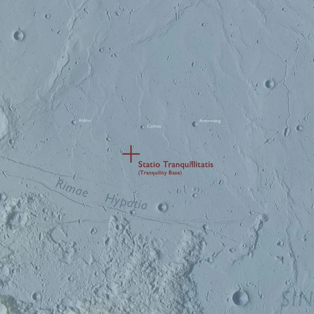
The original requirement that the site be free of craters had to be relaxed and eventually a site within the Sea of Tranquility was chosen.
Tranquillity Base
### Making the map
The first step in creating a map of the Moon was to identify available data that represents the Moon’s topography. The good news is, there are lots of [Digital Elevation Model’s or DEM’s](https://en.wikipedia.org/wiki/Digital_elevation_model) of the Moon, which are 3D representations of a terrain’s surface.
[The United States Geological Survey (USGS) have a 60 metre per pixel DEM](https://astrogeology.usgs.gov/search/map/Moon/LRO/LOLA/Lunar_LRO_LrocKaguya_DEMmerge_60N60S_512ppd) which was created by NASA’s LOLA Team and JAXA’s SELENE/Kaguya Team. From this DEM we were able to create a terrain representation using Geographic Information Software (GIS). After a few issues trying to download the DEM due to the United States Federal Government shutdown, I was eventually able to load it into a GIS, in this case [QGIS](https://www.qgis.org/en/site/). The DEM was projected using the Moon 2000 projection (IAU 2000:30100).
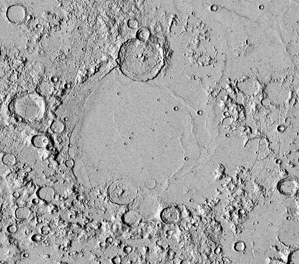
Digital Elevation Model
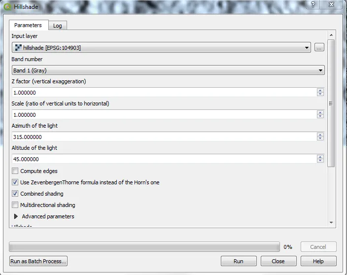
Next, I located the lunar landing site of Apollo 11 and worked out the extent of the Moon around it that I wanted to map. I chose an area of 1350km by 1000km at a scale of 1:1,470,000 and clipped from the original DEM before using it to create hill shade. QGIS has a great GDAL hill shade option that allows you to import your raster (DEM) and output a shaded relief effect based on the parameters you set in the dialogue box.
QGIS hillshade settings
These parameters include:
* Z factor vertical exaggeration – used to emphasise vertical features especially where they might be too small to identify relative to the horizontal scale.
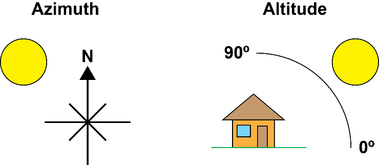
* Azimuth of the light – the angular direction of the sun, measured from north in clockwise degrees from 0 to 360. East = 90, south = 180 and so on.
* Altitude of the light – the angle in degrees of the illumination source from 0 (horizon) to 90 (overhead)
Azimuth and Altitude
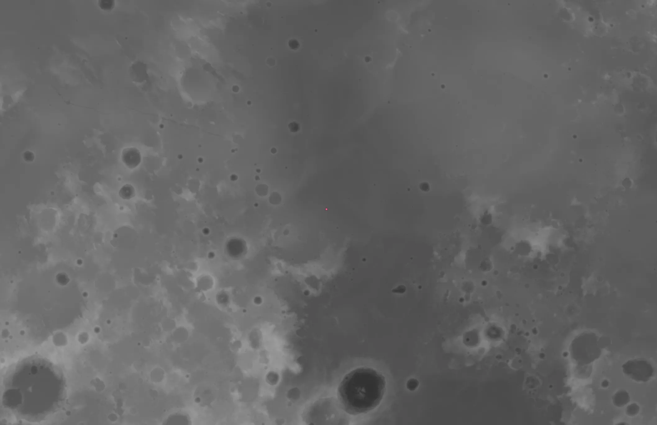
For the purpose of my moon’s hill shade I kept the vertical exaggeration at 1, the azimuth at 315 degrees and altitude at 45 degrees. I opted for the ZevenbergenThorne algorithm rather than Horn’s, as I feel it gives a better and smoother end result.
First hillshade
### Colouring the Moon map
The next stage was to agree a colour scheme for the terrain and investigate the best way to apply this. I eventually settled on a similar palette inspired by a winning photograph for Astronomy Photographer of the Year 2018 which I discovered on the [BBC website](https://www.bbc.co.uk/news/in-pictures-45978380). The photograph is by Jordi Delpeix Borrell and you’ll need to scroll about a third of the way down to find it.
Yellows are used to depict higher areas of terrain whilst blues are used for lower areas. The palette was applied to the original DEM and had a transparency applied before being overlaid on top of my hill shade. The next step was to add some labels which came from the Planetary Nomenclature gazetteer as supplied by NASA and the USGS. The map includes the names of the landing site, craters, lunar mares, bays, mountain ranges, ridges, valleys and trenches.
At this stage the main map topography is complete, but before exporting the map for use in a graphics software, I added a grid depicting both distance and latitude and longitude. This was done using the print composer within QGIS under the Item Properties menu. I then exported the image and grid as an editable PDF that I could then edit within some graphics software, which in this case is Adobe Illustrator. Within Illustrator the map was framed and a grid depicting distance in kilometres added. Alongside this a grid showing latitude and longitude in degrees was added all using the original grids I created in QGIS as a template.
To the south of the map, I created a landscape legend which included, amongst other things, the map title, credits, timeline of the Apollo 11 mission and extent map. The labels were then cartographically positioned and coloured to match the main aesthetics of the map topography.
### More about the OS Moon Map
The map was an absolute joy to make and is something the GDV team are proud of.
You can buy a copy of the map via the [Ordnance Survey shop](https://shop.ordnancesurvey.co.uk/apollo-11-landing-the-moon/).
[We even made an ArcGIS story map.](https://storymaps.arcgis.com/stories/65f55419593744afbec48276c6e5b63c)
---
# Agent Instructions
This documentation is published with GitBook. GitBook is the documentation platform designed so that both humans and AI agents can read, navigate, and reason over technical content effectively. Learn more at gitbook.com.
## Querying This Documentation
If you need additional information that is not directly available in this page, you can query the documentation dynamically by asking a question.
Perform an HTTP GET request on the current page URL with the `ask` query parameter, and the optional `goal` query parameter:
```
GET https://docs.os.uk/more-than-maps/geographic-data-visualisation/geodataviz-assets/how-did-i-make-that/apollo-11-landing.md?ask=&goal=
```
`ask` is the immediate question: it should be specific, self-contained, and written in natural language.
`goal` is optional and describes the broader end goal you are ultimately trying to accomplish on behalf of the user. GitBook uses it to tailor the answer towards what is most useful for that goal.
The response will contain a direct answer to the question and relevant excerpts and sources from the documentation.
Use this mechanism when the answer is not explicitly present in the current page, you need clarification or additional context, or you want to retrieve related documentation sections.