North York Moors National Park, 70 years

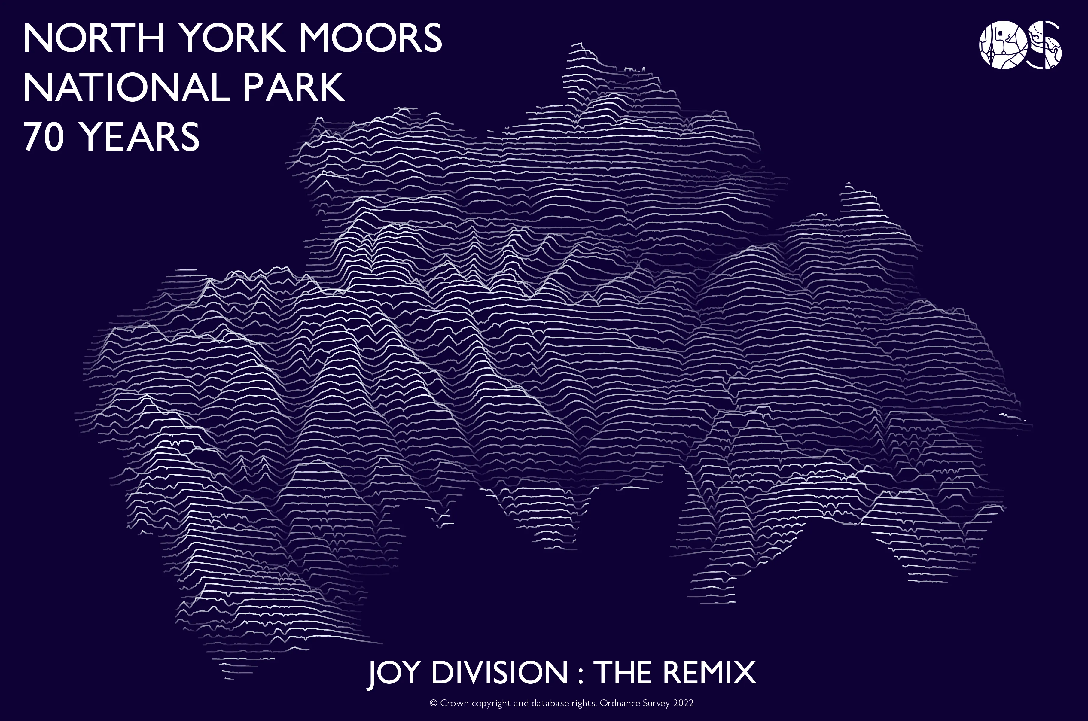
The inspiration for the North York Moors National Park came from Helen Mckenzie’s Blog ‘How to Joyplot’. A joyplot, otherwise known as a ridgeplot, is essentially a series of stacked line graphs. Our final data visualisation was inspired by the album cover of Joy Division’s Unknown Pleasures which was released in 1979. The colours were chosen to mirror the heather of the moors. We followed Helen’s tutorial to create our Joyplot but have explained below how we created our North York Moors Joyplot using OS data, along with how we used Adobe Illustrator to tweak the styling in a simple and effective way.

We have used elevation data from OS Terrain 5 to create a series of elevation profiles to represent the terrain of the North York Moors National Park. This map could be recreated using OS Terrain 50, which is an open dataset. We also use the ‘National Parks’ layer from OS Open Zoomstack to get the national park boundary. To create the map we used QGIS, R Studio and Adobe Illustrator.

Step 1

The relevant ascii grid tiles of OS Terrain 5 were imported into QGIS and merged to create a single elevation model. The main focal point, the North York Moors National Park, was filtered from the National Parks layer of OS Open Zoomstack, with the boundary being used to clip the elevation model.

Step 2

We first created horizontal transects using the following steps:

1. In the top toolbar of QGIS, go to Vector > Research Tools > Create Grid

2. Set the Grid type to ‘line’ and the grid extent calculated from the National Park polygon layer. The horizontal spacing of the lines is not required but we set this to 1000 to make them easier to delete later. We set the vertical spacing to 450m, aiming for close to 100 horizontal lines (the North York Moors National Park is approximately 45km from its most southerly extent to its most northerly extent, give or take a few kilometres).

3. Delete the vertical lines by right clicking on the new grid layer in the layers panel and clicking ‘toggle editing’. Next, select the vertical lines and delete them. Save your edits.

4. Clip the grid to the National Park extent.

Step 3

We then created a point dataset and attributed each point with the elevation data:

1. Open the Processing Toolbox panel. Under Vector creation, select ‘Generate points (pixel centroids) along line’. The raster layer will be your elevation data (in our case the Terrain 5 Elevation Model). The vector layer will be your newly created grid layer. This tool creates a point for every pixel in your elevation dataset along your horizontal transects.

2. Run the tool. You may end up with what looks like a black screen – this is just all the points overlapping. You can change the size of the points by adjusting the layer symbology if you wish.

3. Next, we need to add an elevation to each of these points. You will need to use a plugin for this. In the top toolbar, go to Plugins > Manage and Install Plugins and search for ‘Point Sampling Tool”.

4. Go to the layers panel and ensure your new point layer plus your elevation dataset are turned on (i.e. ticked as visible) as they have to be for the Point Sampling Tool to work.

5. Go to Plugins > Analyses > Point Sampling Tool. The Layer containing sampling points is the new point layer you’ve just created and the layer with fields/bands to get values from is your elevation dataset. You’ll need to specify a file location and name to save this layer in. This may take a little time to run.

6. The final stage is to add coordinates to these points (x and y coordinate). In the Processing Toolbox panel, under Vector Table, select ‘Add X/Y fields to layer’. Your input layer will be the point layer you’ve just created with the elevation attached. Leave the Coordinate system as the default. Run the tool.

7. Now we need to export this data as a csv file for use in R. Right click on your final point layer and go to Export > Save features as. Change the format to ‘Comma Separated Value [CSV]’. Give your file a sensible name such as ‘Points_NorthYorkMoors’.

Step 4

Now we can start creating your joyplot in R Studio.

1. Open RStudio

2. Go to File > New File > R Script. A new window should open titled ‘Untitled’.

3. In this window we want to add our script. You can paste the script below into this window, making sure you change your data source location to where your csv file is saved.

4. When you’re happy, highlight the whole script and click Run at the top right of the script panel. It may take a little while to process but you should see your plot appear in the ‘Plot’ panel. You can change all sorts of things about the way the plot looks using R if you know how. However, for simplicity, you can do the next stage of processing in Adobe Illustrator or similar graphics editing software.

5. Export your joyplot as a PDF.

Step 5

Now we can do some basic editing in Adobe Illustrator or similar graphics package.

1. Open your pdf in Adobe Illustrator

2. Right click on the plot and select ‘Release Clipping Mask’. Each of your lines will now be editable individually.

3. Change the colour of the background to whatever you want. We would recommend putting this background polygon on a separate layer and then lock it.

4. In the layers panel, delete all the black ‘fill’ polygons.

5. You can now trim down the lines at the bottom to better represent the outline of the North York Moors National Park and can adjust the styling of the lines – their thickness and colour – we applied a gradient fill to ours, rotated by -90 degrees.

After Adobe Illustrator

Although we used ggridges in R to create the stacked line graphs, it is also possible to create the same thing using the JoyPy python package.