> For the complete documentation index, see [llms.txt](https://docs.os.uk/more-than-maps/llms.txt). Markdown versions of documentation pages are available by appending `.md` to page URLs; this page is available as [Markdown](https://docs.os.uk/more-than-maps/geographic-data-visualisation/geodataviz-assets/how-did-i-make-that/britains-most-complex-motorway-junctions.md).
# Britain's most complex motorway junctions
Did you know that there are 50 motorways in Great Britain with over 8,300 km of roads and a whopping 666 junctions?
How many junctions have you taken? Or will you be taking as you head off for the summer holidays? Ever tried to come off a motorway junction, only to find you’ve taken the wrong exit and are now heading in the wrong direction? Maybe you’ve driven through the famous ‘Spaghetti Junction’ in Birmingham, and wondered what it looks like from above? Or perhaps you’ve been perplexed at how the most complex of junctions somehow actually work?
Well here at Ordnance Survey, we’ve spent many hours over the years thinking about the interwoven laces of motorway junctions. Not from the perspective of a driver, but that of a cartographer. From data architects conceptually modelling how to capture data, to surveyors capturing the exact GPS locations of our roads, and to the cartographers that digitise the maps you use to travel along the motorways – a lot of thought goes into how to cartographically represent junctions in a way they make sense to the map reader.
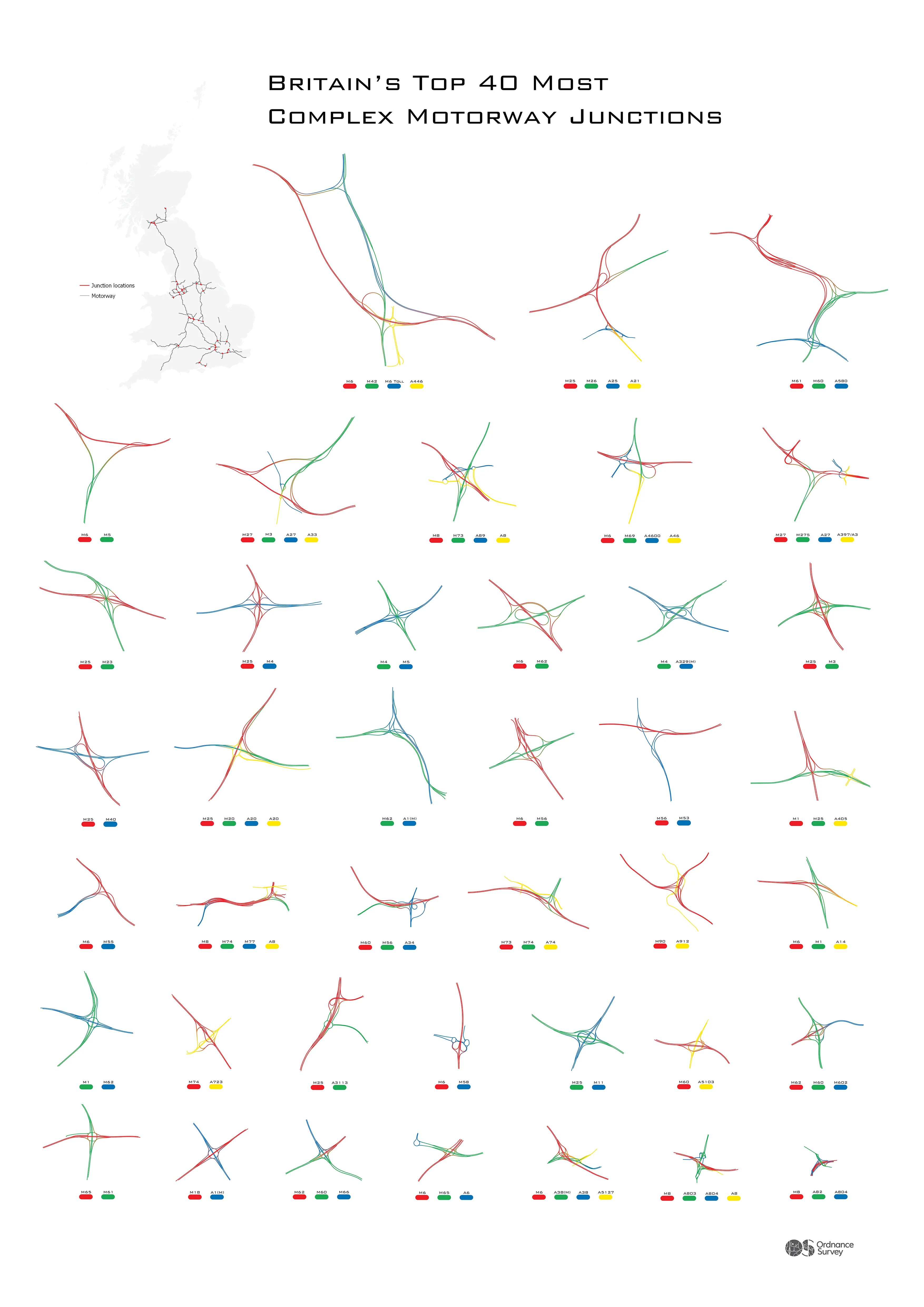
Britain's top 40 most complex motorway junctions
Well here at Ordnance Survey, we’ve spent many hours over the years thinking about the interwoven laces of motorway junctions. Not from the perspective of a driver, but that of a cartographer. From data architects conceptually modelling how to capture data, to surveyors capturing the exact GPS locations of our roads, and to the cartographers that digitise the maps you use to travel along the motorways – a lot of thought goes into how to cartographically represent junctions in a way they make sense to the map reader.
### Cartographically complex motorway junctions
“How can we represent these 3D structures in 2D?”; “Which roads go over which other roads?”; “What colours best represent each of the roads?”; “Where does one road change over into another and how can this be made clear?”; “How can I fit everything in at larger scales?”; “Can you even see what is going on here?”; and “There are so many overlapping line segments…”
As you can imagine, some junctions provide a bigger headache to our cartographers than others. Just as some junctions (although probably not the same ones) are more of a headache to drivers!
Our GeoDataViz team got thinking (even more) about these interwoven laces and how, as difficult they may be to map, there is something mesmerising about them. Getting a bird’s eye view of them and following the individual paths as they weave through what might resemble spaghetti, some sort of flower or a bow-tie. It’s a beauty that cannot be appreciated in the same way from the ground.
It turns out, we aren’t the first to have had thoughts on the, potentially subjective, beauty that lies in these junctions. Many people before us have visualised some of the most complex junctions in the world through truly fantastic graphics. But we wanted to make a GB equivalent and share with you the beauty that lies in what we consider the most cartographically complex motorway junctions. I’m sure there are far more difficult junctions out there to drive, many of which won’t even be found on motorways, but we are focusing on what we know best, the cartography.
### How did we go about choosing these 40 junctions?
More specifically, how did we identify these as being the most complex? Firstly, we decided to focus on motorway junctions only. This makes our search radius easier, but also perhaps more of you will be able to recognise them and even remember driving them. Next, we digitised a buffer around every junction where two or more motorways intersected.
Analytics helped us determine the total number of road nodes, where two road links intersect; the total number of motorway road links; and the combined number of motorway and A–road road links within that buffer. We then pulled out the top 40 junctions that matched each of these three criteria and decided which ones made the cut. Of the three sets, we chose the top 40 junctions with the highest number of overlapping motorway road links, because they really indicated an unrivalled 3D complexity.
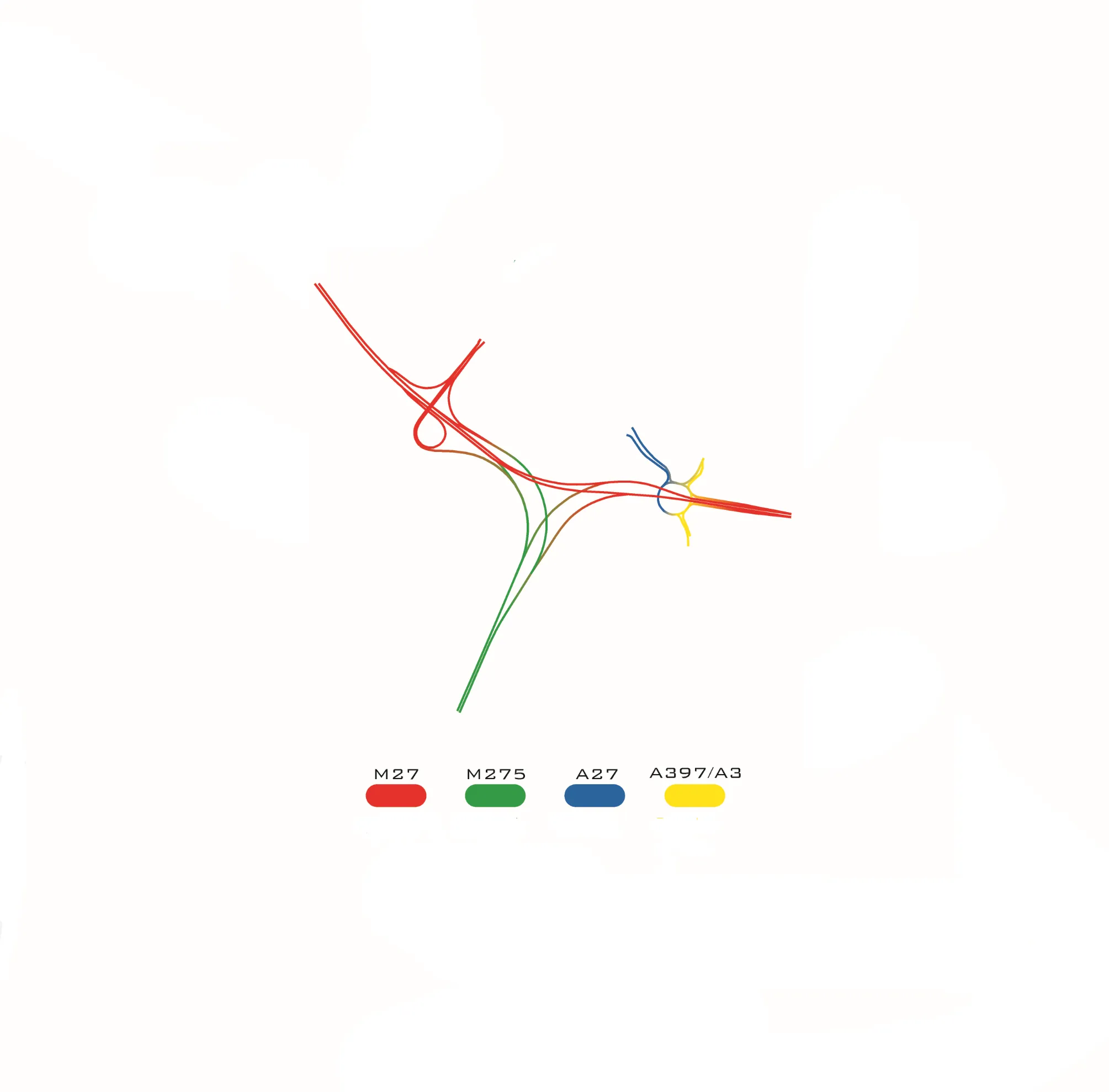
Next we extracted all the motorway and A–road road links that interact with each individual junction within the designated buffer and imported these into Adobe Illustrator, where the real design fun could start. Every road in each junction was assigned a different colour. Making more primary roads either red or green, and secondary roads either blue or yellow. Where one road changes over to another road, a gradient from one colour to the next was used to create the final product.
How many junctions can you recognise?
### See the poster in more detail
The legend under each junction will tell you which road is which colour, but how many junctions can you recognise and label without using the legend at all? And how many of these junctions have you passed through?
**See the full poster and download it in various sizes on our** [**Flickr**](https://www.flickr.com/photos/ordnancesurvey) **page.**
---
# Agent Instructions
This documentation is published with GitBook. GitBook is the documentation platform designed so that both humans and AI agents can read, navigate, and reason over technical content effectively. Learn more at gitbook.com.
## Querying This Documentation
If you need additional information that is not directly available in this page, you can query the documentation dynamically by asking a question.
Perform an HTTP GET request on the current page URL with the `ask` query parameter, and the optional `goal` query parameter:
```
GET https://docs.os.uk/more-than-maps/geographic-data-visualisation/geodataviz-assets/how-did-i-make-that/britains-most-complex-motorway-junctions.md?ask=&goal=
```
`ask` is the immediate question: it should be specific, self-contained, and written in natural language.
`goal` is optional and describes the broader end goal you are ultimately trying to accomplish on behalf of the user. GitBook uses it to tailor the answer towards what is most useful for that goal.
The response will contain a direct answer to the question and relevant excerpts and sources from the documentation.
Use this mechanism when the answer is not explicitly present in the current page, you need clarification or additional context, or you want to retrieve related documentation sections.