Famous shipwrecks of Pembrokeshire

As Pembrokeshire is a coastal national park, for this map it felt right to incorporate some sort of ocean-based data. Pembrokeshire has a large number of shipwrecks around its coast – partly caused by some very large storms occurring in 1703 and 1859. It also has varied sea and wind conditions, and many dangerous rock formations which left historical sail ships at the mercy of the weather conditions. This map by no means shows all of those shipwrecks – some divers and historians believe there are thousands of them dotted in the waters around Pembrokeshire.

This map was made with a combination of Ordnance Survey (OS) and UK Hydrographic Office (UKHO) data. The UKHO data portal includes some great opensource datasets and it’s a good opportunity to extend the map beyond ‘The Extent of the Realm’ of Great Britain (up to the coastline) which is as far as Ordnance Survey mapping goes. The UKHO also have bathymetric elevation profiles which can be downloaded for free – I think they would look great on a future OS map.

The process of making this map combined a few different techniques.

I completed this map using QGIS, Adobe Photoshop, and Adobe Illustrator - although other software such as ArcGIS or ArcPro could also be used instead of QGIS.

First off, I started with a Digital Elevation Model (DEM) of Great Britain – using OS Terrain 50 data. I then clipped this to the National Park area, to highlight the elevation of the land in Pembrokeshire. I styled the DEM using a singleband pseudo colour effect – picking out this turquoise shade for the colour scheme of my map. I chose to represent the low-lying areas with darker shades, and the higher elevations with lighter colours to give that really nice hillshade effect. I then applied a transparency to the DEM of the whole country, making it more washed out and allowing the terrain of the National Park to stand out.

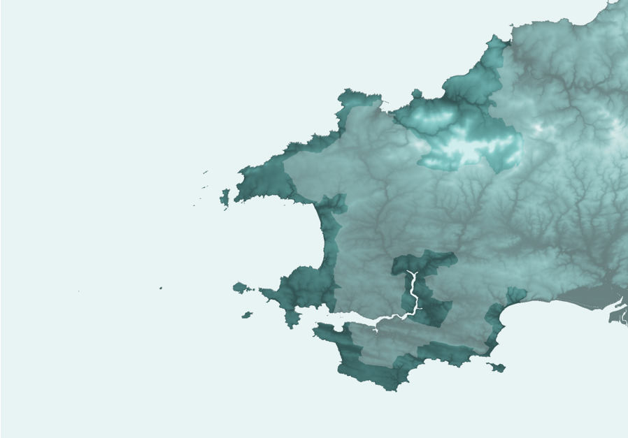
A Digital Elevation Model was used to create the first layer of the Pembrokeshire shipwreck map.

Next, I imported the ‘Shipwrecks and Obstructions’ dataset from the UKHO. This is a global opensource dataset that can be found here, with over 94,000 points, so I clipped it to my study area so I wasn’t dealing with huge file sizes. It’s worth noting that not all the ‘X’ points in the sea are shipwrecks – some of these represent ‘Obstructions’ such as sunken rocks or pinnacles. To visualise these points I created a custom SVG image file in Adobe Photoshop of a hand-drawn ‘X marks the spot’. I then imported this into QGIS, and used the ‘Raster Image’ point marker function to mark out all of these locations around the Pembrokeshire coast.

The UKHO's ‘Shipwrecks and Obstructions’ dataset was used to pinpoint all the Xs in the Celtic Sea.

I then wanted to add buffer lines extending out from the coast, which are reminiscent of the style of old nautical charts and maps. I used this tool created by John Nelson to calculate buffer distances which give this logarithmic effect, almost as if they are ripples expanding out from the coast. A turquoise fill and white outline for those buffer polygons ties them in nicely with the colour scheme of the rest of the map.

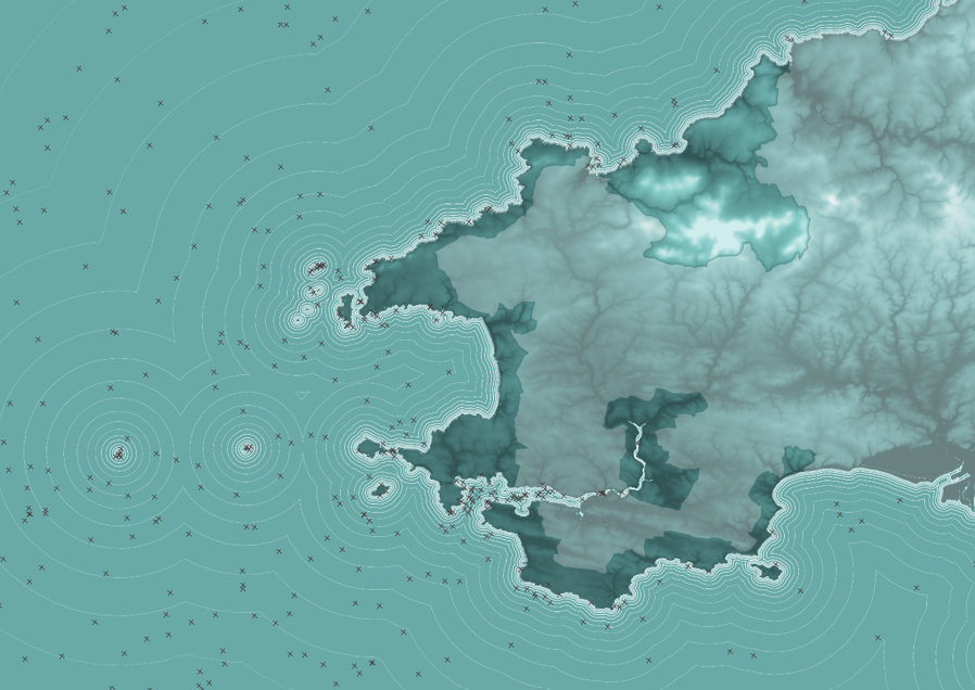
Buffer lines were added to create a ripple effect.

At this point, I was ready to start adding some labels and information about the different shipwrecks dotted around Pembrokeshire’s coast. I didn’t know much about shipwrecks before this – so it involved some research into the history of the area, and identifying specific shipwrecks then locating from historical accounts and vague descriptions whereabouts they are on the map! A lot of credit for the information included in this map goes to James Phillips – a diver who has done a huge amount of work in discovering and documenting shipwrecks around Pembrokeshire. You can read more about his work here.

I then exported my map from QGIS, and brought it into Adobe Illustrator. Here, I added labels for Pembrokeshire National Park and St. Brides Bay, as well as the shipwrecks themselves and added things like leader lines and our logo.

After a few final tweaks, the map was ready to publish!

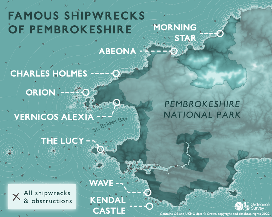
Final map of Pembrokeshire with all labels added.